Understanding the EXECUTION PLAN and it's Components

Understanding the EXECUTION PLAN

To know how Execution Plan helps in Optimizing SQLs- Click here.

In order to determine if you are looking at a good execution plan or not, you need to understand how the Optimizer determined the plan in the first place. You should also be able to look at the execution plan and assess if the Optimizer has made any mistake in its estimations or calculations, leading to a suboptimal plan. The components to assess are:

• Cardinality– Estimate of the number of rows coming out of each of the operations.

• Access method – The way in which the data is being accessed, via either a table scan or index access.

• Join method – The method (e.g., hash, sort-merge, etc.) used to join tables with each other.

• Join type – The type of join (e.g., outer, anti, semi, etc.).

• Join order – The order in which the tables are joined to each other.

• Partition pruning – Are only the necessary partitions being accessed to answer the query?

• Parallel Execution – In case of parallel execution, is each operation in the plan being conducted in parallel? Is the right data redistribution method being used?

Cardinality

 The cardinality is the estimated number of rows that will be returned by each operation. The Optimizer determines the cardinality for each operation based on a complex set of formulas that use both table and column level statistics as input (or the statistics derived by dynamic sampling).

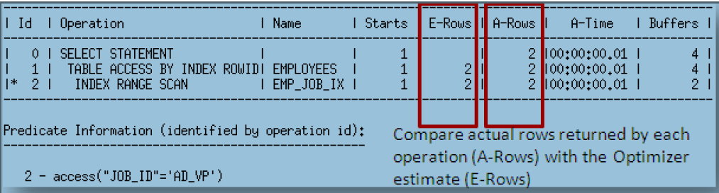
The CARDINALITY estimate is found in the Rows column of the execution plan

Consider Employee Table below having 107 rows.

SQL> SELECT EMP_ID, ENAME, JOB_ID

FROM Employees

WHERE JOB_ID = ‘AD_VP’;

The JOB_ID column has 19 distinct values so the optimizer predicted the cardinality for this statement

to be 107/19 or 5.6 rows, which gets rounded up to 6 rows.

Determine the correct cardinality

To manually determine if the Optimizer has estimated the correct cardinality (or is in close proximity)

you can use a simple SELECT COUNT(*) query for each tables used in the query and applying any

WHERE clause predicates belonging to that table in the query. For the simple example used before

SQL> SELECT COUNT(*)
FROM Employees WHERE JOB_ID=’AD_VP’;
COUNT(*)
-------------
2

Alternatively, you can use the GATHER_PLAN_STATISTICS hint in the SQL statement to automatically collect more comprehensive runtime statistics. This hint records the actual cardinality.

Runtime cardinality statistics are displayed in the A-Rows column

SQL> SELECT /*+ GATHER_PLAN_STATISTICS */ EMP_ID, ENAME, JOB_ID

FROM Employees WHERE JOB_ID = ‘AD_VP’;

Access Method

The access method - or access path - shows how the data will be accessed from each table (or index).

The access method is shown in the operation field of the explain plan.

Oracle supports following common access methods:

Full table scan - Reads all rows from a table and filters out those that do not meet the where clause predicates. A full table scan is selected if a large portion of the rows in the table must be accessed, no indexes exist or the ones present can’t be used or if the cost is the lowest.

Table access by ROWID – The ROWID of a row specifies the data file, the data block within that file, and the location of the row within that block. Oracle first obtains the ROWIDs either from a WHERE clause predicate or through an index scan of one or more of the table's indexes. Oracle then locates each selected row in the table based on its ROWID and does a row-by-row access.

Index unique scan – Only one row will be returned from the scan of a unique index. It will be used when there is, an equality predicate on a unique (B-tree) index or an index created as a result of a primary key constraint.

Index range scan – Oracle accesses adjacent index entries and then uses the ROWID values in the index to retrieve the corresponding rows from the table. An index range scan can be bounded or unbounded. It will be used when a statement has an equality predicate on a non-unique index key, or a non-equality or range predicate on a unique index key. (=, <, >,LIKE if not on leading edge). Data is returned in the ascending order of index columns.

Index range scan descending – Conceptually the same access as an index range scan, but it is used when an ORDER BY .. DESCENDING clause can be satisfied by an index.

Index skip scan - Normally, in order for an index to be used, the prefix of the index key (leading edge of the index) would be referenced in the query. However, if all the other columns in the index are referenced in the statement except the first column, Oracle can do an index skip scan, to skip the first column of the index and use the rest of it. This can be advantageous if there are few distinct values in the leading column of a concatenated index and many distinct values in the non-leading key of the index.

Full Index scan - A full index scan does not read every block in the index structure, contrary to what its name suggests. An index full scan processes all of the leaf blocks of an index, but only enough of the branch blocks to find the first leaf block. It is used when all of the columns necessary to satisfy the statement is in the index and it is cheaper than scanning the table. It uses single block IOs. It may be used in any of the following situations:

• An ORDER BY clause has all of the index columns in it and the order is the same as in the index (can also contain a subset of the columns in the index).

• The query requires a sort merge join and all of the columns referenced in the query are in the index.

• Order of the columns referenced in the query matches the order of the leading index columns.

• A GROUP BY clause is present in the query, and the columns in the GROUP BY clause are present in the index.

Fast full index scan - This is an alternative to a full table scan when the index contains all the columns that are needed for the query, and at least one column in the index key has the NOT NULL constraint. It cannot be used to eliminate a sort operation, because the data access does not follow the index key. It will also read all of the blocks in the index using multiblock reads, unlike a full index scan.

Index join – This is a join of several indexes on the same table that collectively contain all of the columns that are referenced in the query from that table. If an index join is used, then no table access is needed, because all the relevant column values can be retrieved from the joined indexes. An index join cannot be used to eliminate a sort operation.

Bitmap Index – A bitmap index uses a set of bits for each key value and a mapping function that converts each bit position to a ROWID. Oracle can efficiently merge bitmap indexes that correspond to several predicates in a WHERE clause, using Boolean operations to resolve AND and OR conditions.

If the access method you see in an execution plan is not what you expect, check the cardinality estimates for that object are correct and the join order allows the access method you desire.

Join method

The join method describes how data from two data producing operators will be joined together. You can identify the join methods used in a SQL statement by looking in the operations column in the explain plan.

Join Method is shown in the Operations column

Oracles offers several join methods and join types.

Hash Joins - Hash joins are used for joining large data sets. The optimizer uses the smaller of the two tables or data sources to build a hash table, based on the join key, in memory. It then scans the larger table, and performs the same hashing algorithm on the join column(s). It then probes the previously built hash table for each value and if they match, it returns a row.

Nested Loops joins - Nested loops joins are useful when small subsets of data are being joined and if there is an efficient way of accessing the second table (for example an index look up). For every row in the first table (the outer table), Oracle accesses all the rows in the second table (the inner table).

Consider it like two embedded FOR loops. In Oracle Database 11g the internal implementation for nested loop joins changed to reduce overall latency for physical I/O so it is possible you will see two NESTED LOOPS join in the operations column of the plan, where you previously only saw one on earlier versions of Oracle.

Sort Merge joins – Sort merge joins are useful when the join condition between two tables is an inequality condition such as, <, <=, >, or >=. Sort merge joins can perform better than nested loop joins for large data sets. The join consists of two steps:

Sort join operation: Both the inputs are sorted on the join key.

Merge join operation: The sorted lists are merged together.

Cartesian join - The optimizer joins every row from one data source with every row from the other data source, creating a Cartesian product of the two sets. Typically, this is only chosen if the tables involved are small or if one or more of the tables does not have a join conditions to any other table in the statement. Cartesian joins are not common, so it can be a sign of problem with the cardinality estimates, if it is selected for any other reason. Strictly speaking, a Cartesian product is not a join.

Join Types

Oracle offers several join types: inner join, (left) outer join, full outer join, anti-join, semi join, grouped outer join, etc. Note that inner join is the most common type of join; hence the execution plan does not specify the key word “INNER’.

Outer Join - An outer join returns all rows that satisfy the join condition and also all of the rows from the table without the (+) for which no rows from the other table satisfy the join condition. For example, T1.x = T2.x (+), here T1 is the left table whose non-joining rows will be retained. In the ANSI outer join syntax, it is the leading table whose non-join rows will be retained. The same example can be written in ANSI SQL as T1 LEFT OUTER JOIN T2 ON (T1.x = T2.x);

Example plan output using OUTER JOIN. Note a join type is always matched with one of the join methods; in this case a hash join

Join Order

The join order is the order in which the tables are joined together in a multi-table SQL statement. To determine the join order in an execution plan look at the indentation of the tables in the operation column. In Figure 22 below the SALES and PRODUCTS table are equally indented and both of them are more indented than the CUSTOMERS table. Therefore, the SALES and PRODUCTS table will be joined first using a hash join and the result of that join will then be joined to the CUSTOMERS table.

Example plan output highlighting the JOIN ORDER

The join order is determined based on cost, which is strongly influenced by the cardinality estimates and the access paths available. 

The Optimizer will also always adhere to some basic rules:

• Joins that result in at most one row always go first. The Optimizer can determine this based on UNIQUE and PRIMARY KEY constraints on the tables.

• When outer joins are used, the row preserving table (table without the outer join operator) must come after the other table in the predicate (table with the outer join operator) to ensure all of the additional rows that don’t satisfy the join condition can be added to the result set correctly.

• When a subquery has been converted into an antijoin or semi join, the tables from the subquery must come after those tables in the outer query block to which they were connected or correlated. However, hash antijoins and semi joins are able to override this ordering condition under certain circumstances.

• If view merging is not possible all tables in the view will be joined before joining to the tables outside the view.

If the join order is not what you expect check the cardinality estimates for each of the objects and the

access methods are correct.

Partitioning

Partitioning allows a table, index or index-organized table to be subdivided into smaller pieces. Each piece of the database object is called a Partition. Partition pruning or Partition elimination is the simplest means to improve performance using Partitioning. For example, if an application has an ORDERS table that contains a record of all orders for the last 2 years, and this table has been partitioned by day, a query requesting orders for a single week would only access seven partitions of the ORDERS table instead of 730 partitions (the entire table).

Partition pruning is visible in an execution plan in the PSTART and PSTOP columns. The PSTART column contains the number of the first partition that will be accessed and PSTOP column contains the number of the last partition that will be accessed1. In Figure 24 four partitions from SALES are accessed, namely partitions 9,10,11, and 12.

Example plan output highlighting Partition pruning for a single-level partitioned table

A simple select statement that was run against a table that is partitioned by day and sub-partitioned by hash on the CUST_ID column is shown. In this case a lot more numbers appear in the PSTART, PSTOP columns. What do these additional numbers mean?

Example plan output highlighting Partition pruning for a composite partitioned table

When using composite partitioning, Oracle numbers each of the partitions from 1 to n (absolute partition numbers). For a table that is partitioned on just one level, these absolute numbers represent the actual physical segments on disk of the single-level partitioned table.

In the case of a composite partitioned table, however, a partition is a logical entity and not represented on disk. Each partition is subdivided into so-called sub-partitions. Each sub-partition within a partition is numbered from 1 to m (relative sub-partition number within a single partition). Finally, all of the sub partitions in a composite-partitioned table are given a global number 1 to (n X m) (absolute sub partition numbers); these absolute numbers represent the actual physical segments on disk of the composite partitioned table.

Numbering scheme for a partitioned table

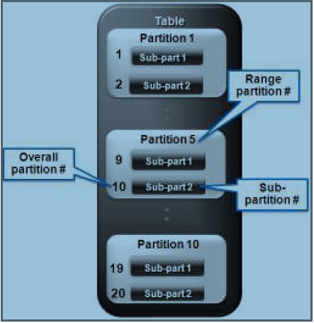
So, in the previous plan in Figure the number 10 in PSTART and PSTOP column, on line 4 of the plan represents the global partitioning number representing the physical segments on disk. The number 5 in PSTART and PSTOP column, on line 2 of the plan represents the partition number; the number 2 in PSTART and PSTOP column, on line 3 of the plan, represents the relative sub-partition number within a partition.

There are cases when a word or letters appear in the PSTART and PSTOP columns instead of a number. For example, you may see the word KEY appears in these columns. This indicates that it was not possible at parse time to identify, which partitions would be accessed by the query but the Optimizer believes that partition pruning will occur at execution time (dynamic pruning). This happens when there is an equality predicate on the partitioning key column that contains a function. For example TIME_ID = SYSDATE. Another situation where dynamic pruning can occur is when there is a join condition on the partitioning key column in the query and the table that is joined with the partitioned table is expected not to join with all partitions, for example because of a FILTER predicate.

Partition pruning will occur at execution time. In the example in Figure27 below the where clause predicate is on the TIME table, which joins to the SALES table on the partition key time_id. Partition pruning will happen at execution time after the WHERE clause predicate has been applied to the TIME table and the appropriate TIME_IDs have been select.

Example plan output highlighting dynamic Partition pruning

If partition pruning does not occur as expected, check the predicates on the partition key column. Ensure that the predicates are using the same datatype as the partition key column. You can check this in the predicate information section under the plan. If the table is hash partitioned, partition pruning will only occur if the predicate on the partition key column is an equality or an in-list predicate. 

Also, if the table has multi-column hash partitioning then partition pruning will only occur if there is a predicate on all columns used in the hash partitioning.

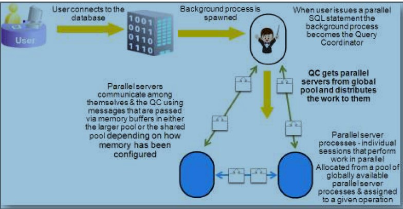
Parallel Execution

Parallel execution in the Oracle Database is based on the principles of a coordinator (often called the Query Coordinator or QC for short) and parallel server processes. The QC is the session that initiates the parallel SQL statement and the parallel server processes are the individual sessions that perform work in parallel. The QC distributes the work to the parallel server processes and may have to perform a minimal, mostly logistical, portion of the work that cannot be executed in parallel. 

For example, a parallel query with a SUM() operation requires adding the individual sub-totals calculated by each parallel server processes.

Concept of parallel execution in the Oracle database

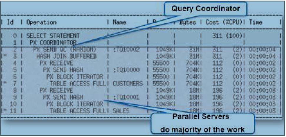
The QC is easily identified in the parallel execution plan as it writes its name in the plan. You can see this on the line with ID#1 of the plan shown in Figure where you see the operation 'PX COORDINATOR'. All of the operations that appear above this line in the execution plan are done by the QC. Since this is a single process all of these operations are done serially. Typically, you want to minimize the number of operations done by the QC. All of the operations done under the line ‘PX COORDINATOR’ are typically done by the parallel server processes.

Example plan output highlighting the concepts of parallel execution